Experimenting with image filters and blending techniques
Background
In this project, we explore various use cases of filters/convolution and the frequency domain of images. Part 1 (and Part 2.1) explores various edge detection schemes using filters and Part 2 mainly uses the frequency domain of images to perform some interesting tasks.
Part 1: Filters
1.1 Finite Difference Operator
First, we use the simple finite difference operators to perform edge detection on the cameraman image. In particular, we convolve the filters D_x = [-1 1] and D_y = [1 -1]^T^ with the cameraman image to get the partial derivatives of the x and y directions, as shown below. To combine this into one edge-detected image, we perform a gradient magnitude computation as follows: res(i,j) = sqrt(cameraman_dx(i,j)^2^ + cameraman_dy(i,j)^2^) where res is the output image, cameraman_dx is the convolution of the cameraman image with D_x, and cameraman_dy is the convolution with D_y. This uses the partial derivatives of the x and y directions to find the gradient magnitude for the image. As seen below, this creates a better edge detection overall that accounts for edges in all directions. Finally, to make the edge detection more clear, we binarize the gradient magnitude image by setting all pixels above 50 to 255 and pixels at or below 50 to 0. We tested out different thresholds and found 50 worked well.

1.2 Derivative of Gaussian (DoG) Filter
With the finite difference operator, the results were a little noisy and had jagged edges, as seen in the binarized image. To get smoother edge detection, we blur the original image by convolving it with a 2D gaussian kernel, then performing the same edge detection scheme with the finite difference operators.

As seen in the images above, there are clear differences between naively applying the finite difference filters (like in part 1.1) and blurring with a gaussian filter first then applying the finite difference filters. The edge-detected images from this part are much smoother than in the previous part, especially in the binarized images. The camerman no longer has jagged edges and instead has smooth, continuous edges. Furthermore, using the properties of convolution, we can combine the blurring and derivative filters into a single filter called the Derivative of Gaussian filter (DoG) which we only need to convolve once with the cameraman image to perform smooth edge-detection. The results of applying the DoG filter are shown below; notice they are exactly the same as the images above.

Part 2: Frequencies
2.1 Image Sharpening
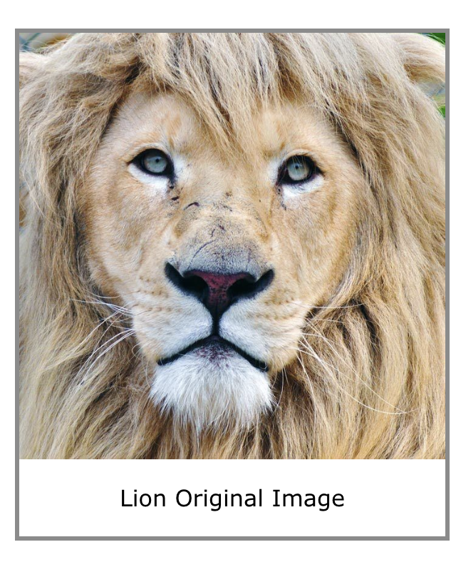
Now we try to use filters to sharpen an image, which means making the edges more “defined”. To do this, we get the high frequencies of an image by applying a gaussian filter to blur the image (i.e get the low frequencies) then subtracting the blurred image from the original image. This leaves only the high frequencies (mostly edges) which we then add back to the original image to obtain a sharpened image. We also use a parameter alpha which controls how much the image is sharpened. Mathematically, sharpened_image(i,j) = alphaoriginal_image(i,j) + (alpha-1)blurred_image(i,j). Furthermore, we can combine the gaussian filter and subtraction into a single filter called the unsharp mask filter by computing alphae - (alpha-1)gaussian_filter, where e is the unit impulse (a kernel with 1 in the middle and zeros elsewhere). The progression of sharpening some images is shown below.


For evaluation purposes, we also blurred an image and tried to sharpen it again. The results are shown below:

2.2 Hybrid Images
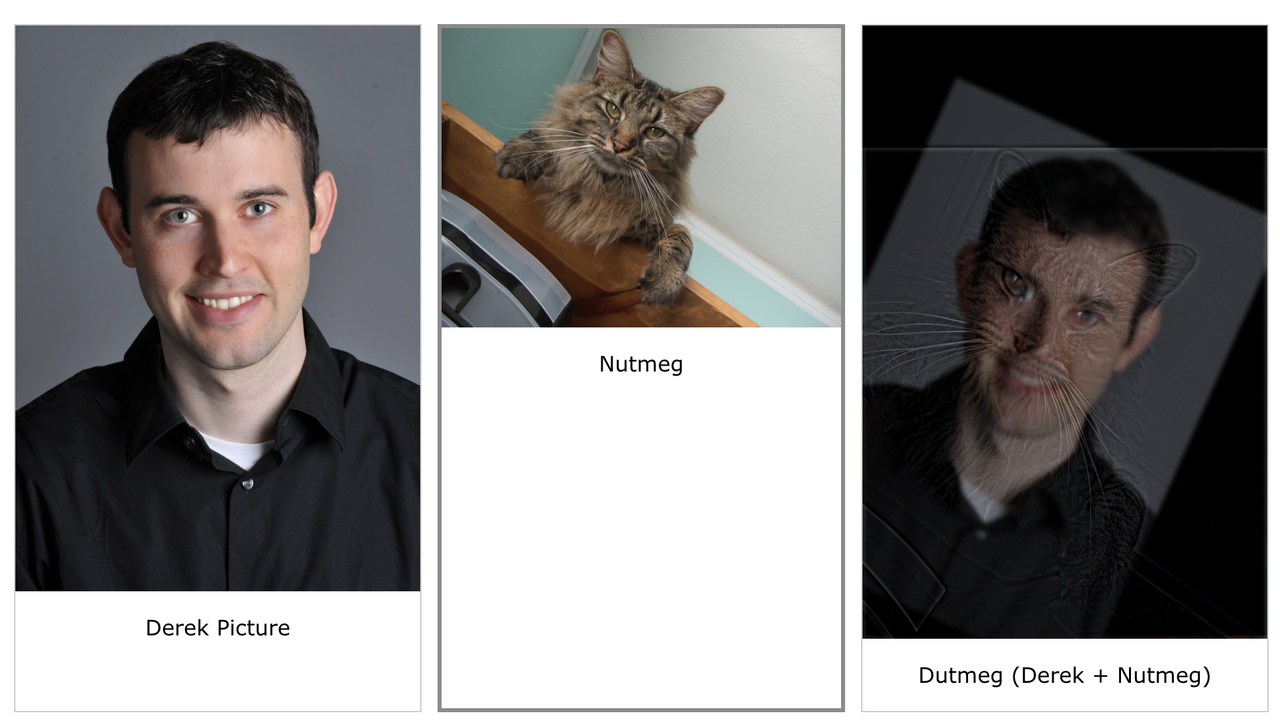
To create hybrid images, we combined the low frequencies from one image with the high frequencies from another. In particular, to compute the low frequencies for image A, we convolved image A with a gaussian kernel to blur it. To compute the high frequencies for image B, we computed the low frequencies using a gaussian kernel and subtracted it from the original image. Then we averaged the low frequency image A with the high frequency image B to get the hybrid image. We had to experiment with the kernel sizes and the sigmas (cutoff frequencies) for each gaussian filter to get the most aesthetically pleasing result.

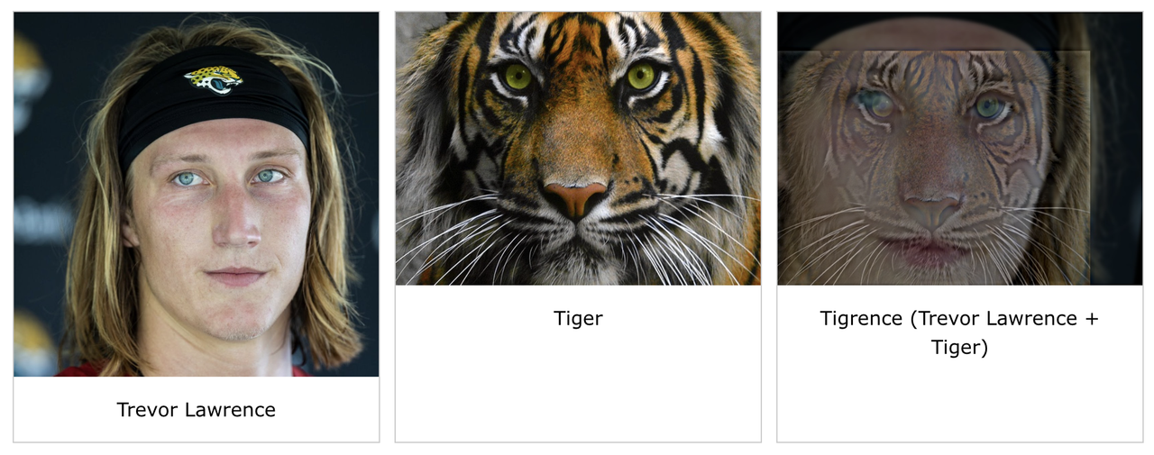
Here are the FFT plots for the Tigrence hybrid image:

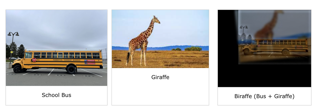
Here is an example of a failed hybrid image, a school bus and a giraffe. The school bus is too short for the giraffe so the output looks strange:
2.3 Gaussian and Laplacian Stacks
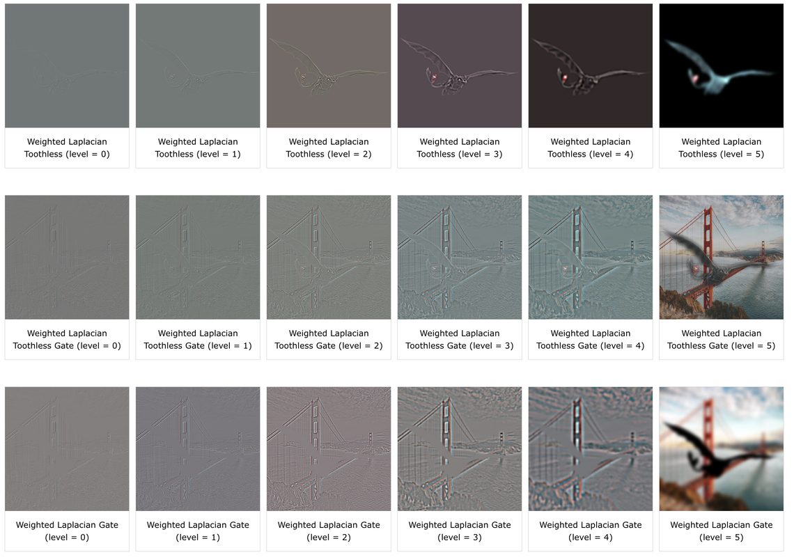
We used Gaussian and Laplacian Stacks to blend an apple and an orange image. In our procedure, we first created the gaussian stacks for the apple and the orange by successively blurring the images with gaussian filters that doubled in sigma at each level. We had 6 levels overall. Then, to create the laplacian stacks for these images, we subtracted consecutive levels of the gaussian stacks (i.e. gaussian_stack[i] - gaussian_stack[i+1]). Furthermore, we made the gaussian stack for the mask as well. Finally, to blend the image, we created a laplacian stack for the output via the formula laplacian_output(i,j) = gaussian_mask(i,j)laplacian_apple(i,j) + (1-gaussian_mask(i,j))laplacian_orange(i,j) at each level. That is, we weight the laplacians of both images by the gaussian of the mask at each level. To get the output image, we collapse the output laplacian stack by summing across all the levels. The result is a smoothly blended oraple.


2.4 Multiresolution Blending
We also selected our own images to blend and used irregular masks during the blending process. We followed the same procedure for blending as outlined in the previous section for the oraple, except now with irregular masks. For example, here is the blending process of an image of Toothless (the dragon from “How to Train your Dragon”) and an image of SF’s Golden Gate Bridge:

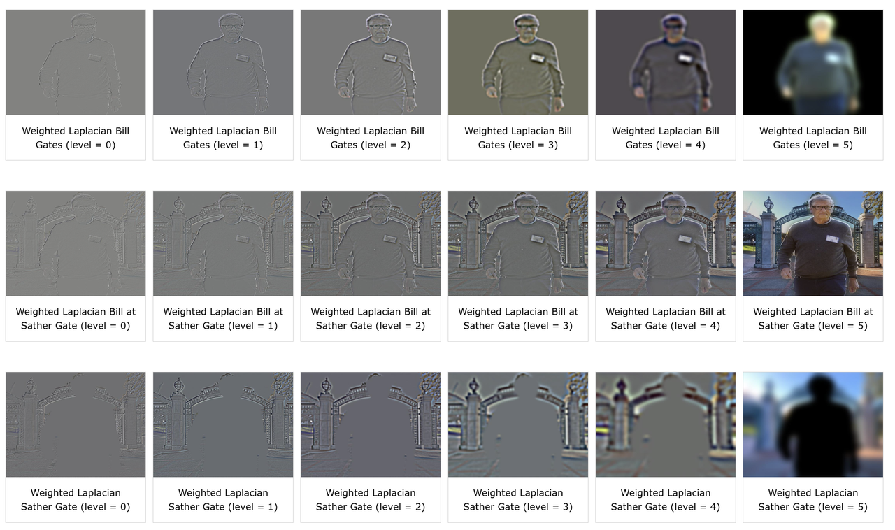
Here is the blending process of an image of Bill Gates walking and an image of Sather Gate at UC Berkeley. The blended image shows Bill walking in Sather Gate:

