Background

In this project, we explore how a neural radiance field (NeRF) can be used to represent 3D space. A NeRF is a function F: {x,y,z,θ,φ}→{r,g,b,σ} that takes in world coordinates x,y,z and a viewing direction θ,φ and returns a color value r,g,b and density σ that is used to create a 2D projection of the world from that perspective. This function is found by training a neural network. In part 1, we consider a simple case of a NeRF for a 2D image and, in part 2, we train a deeper neural network to represent a 3D space

Part 1: Fitting a Neural Radiance Field to a 2D Image

To understand radiance fields, we consider a simple NeRF F: {u,v} → {r,g,b} that maps 2D pixel coordinates to a color value. We train a shallow neural network to learn this function on an image and optimize it to reconstruct the image. We use the MLP architecture shown below, with a sigmoid activation at the end to ensure the RGB values lie in the normalized range (0,1). Furthermore, to enable local pixels to have sufficient variability in their RGB values, we use positional encoding. A series of sinusoidal functions is applied to the 2D input coordinates to expand its dimensionality to 42. We also normalized the pixels values and pixel coordinates before training the network. In training the network, for each iteration, we sample a batch of 10,000 random pixels from the image, using the pixel coordinates as the input and known RGB values for each pixel as the target. Our loss function is the peak signal-to-noise ratio (PSNR).

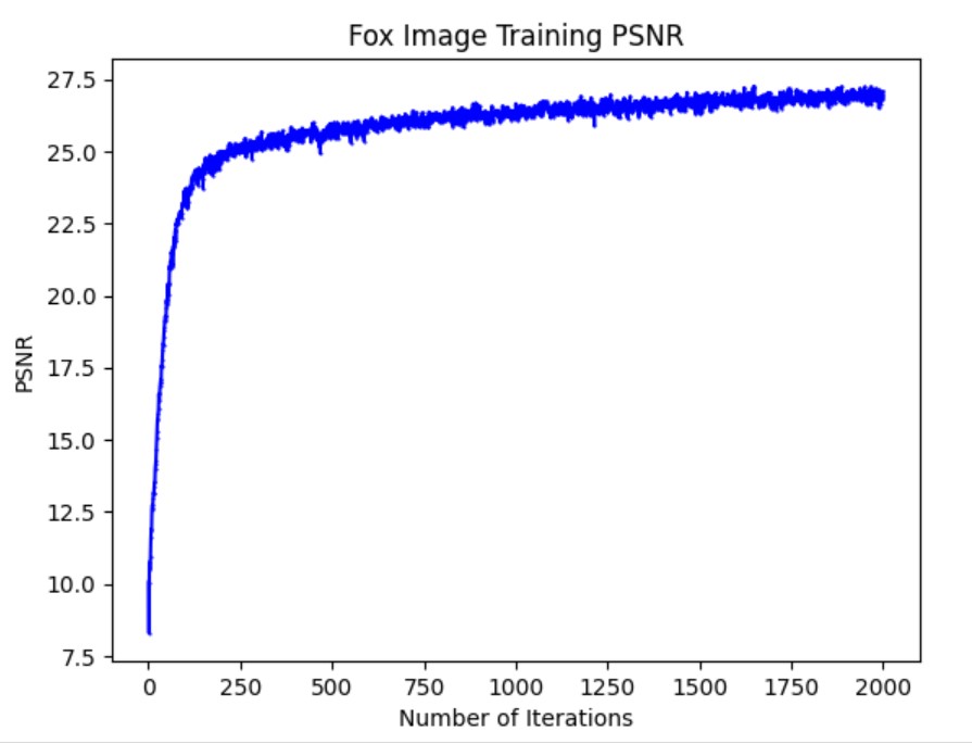
The training PSNR and predicted images across intermediate iterations are shown below. The hyperparameters used were: batch_size = 10000, learning_rate = 1e-2, L = 10, number_of_layers = 4, channel_size = 256. Overall, the model reconstructs the image pretty well but it is still a little blurry compared to the original image. Perhaps more iterations are needed to allow the model to learn higher dimensional features

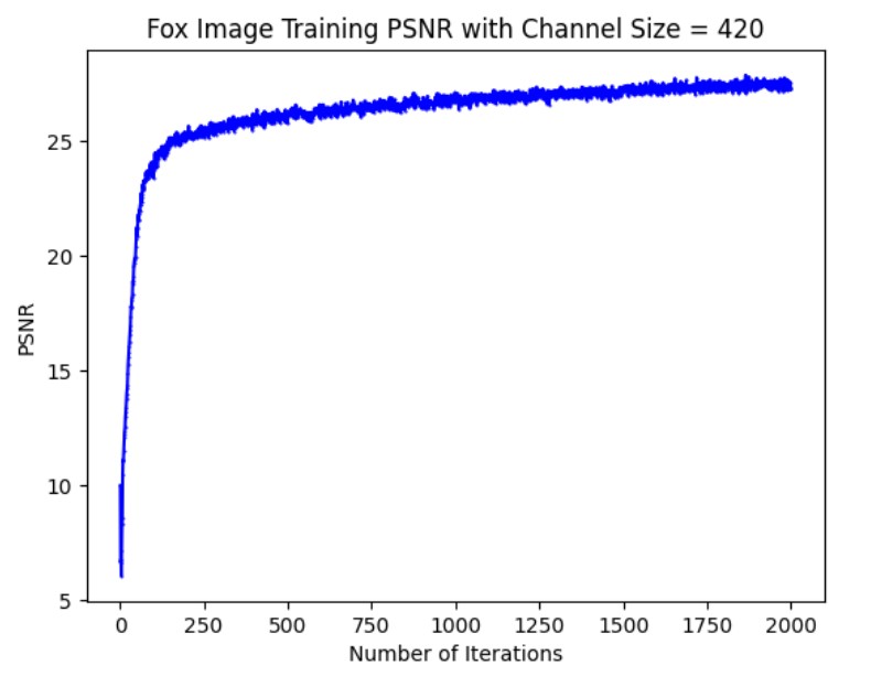
We also changed the channel size hyperparameter from 256 to 420 to see how the performance is affected. This caused the model to perform worse and get a lower PSNR, perhaps because more iterations are needed to correctly update all the weights. The final fox image looks okay but is blurrier than the predicted image with the original hyperparameters

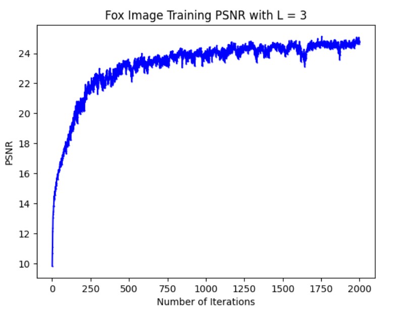
Additionally, we changed the hyperparameter for the length of the positional encoding, L from 10 to 3. This caused the performance to be signifcantly worse, as seen in the predicted images across iterations. The model is much slower in converging to a high PSNR so the final result after 2000 iterations is much blurrier. This is probably because, with a lower dimsional positional encoding, it takes longer for the model to discrimiate colors for pixels that are spatially close

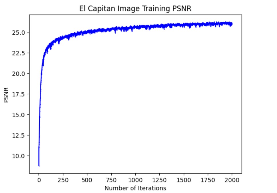
Finally, we optimized this model to reconstruct an image of El Capitan in Yosemite National Park. The hyperparameters used were: batch_size = 30000, channel_size = 300, L = 15, number_of_layer = 4, learning_rate = 1e-2. Overall, the model fit the image well and reconstructs most of it with a good PSNR.

Pat 2: Fitting a Neural Radiance Field to Multi-View Images

Now that we understand the basics of NeRFs, we train a deeper NeRF to represent the 3D space of a lego truck. There are a number of preprocessing and postprocessing steps we implement to train this more complex model

Create Rays from Cameras

First, we write functions to convert between pixel, camera, and world coordinates and create rays from a pixel. To convert from camera to world coordinates, we create a function that takes in a camera-to-world (c2w) matrix and a coordinates tensor of shape (batch_size, 3). A column of ones is appended to the coordinates tensor (to allow affine transformations) then it is tranposed and multiplied with the c2w matrix to generate the world coordinates. To convert from pixel to camera coordinates, a similar process is employed, except we multiply by the inverse of the intrinsic matrix K and a depth s to get 3D coordinates in the camera system. Finally, we write a function to create rays from 2D pixel coordinates. The origin of the rays is found by converting the camera coordinates [0,0,0] to world coordinates (i.e. we multiply the c2w matrix by the vector [0,0,0,1]). And the ray direction for each pixel (u,v) is found by first converting the pixel to camera coordinates, then world coordinates to get X~w~ = (x~w~ y~w~ z~w~). We then use the formula r~d~ = (X~w~-r~0~) / X~w~-r~0~~2~ where r~0~ is the ray origin to get the normalized ray direction. All of these functions support batched coordinates by taking in a tensor of shape (batch_size,3), i.e. the coordinates are laid out in rows.

Sampling

Next we implement random sampling to get rays from different perspectives. First, we write a function sample_rays which uses a set of images and corresponding c2w matrices and returns a sampling of N ray origins, ray directions, and RGB values from the pixels across all images. We do this by sampling M random images, then sampling N//M random rays from each image, keeping track of what the actual RGB values for each ray are for training purposes. We found that the values N = 10000, M = 50 worked pretty well in producing a low PSNR. We also wrote a function sample_along_rays which takes in a set of ray origins and ray directions and discretizes each ray by sampling evenly at points along the ray. Namely, we sample 64 points evenly from 2.0 to 6.0 (i.e. t = np.linspace(2.0,6.0,64)) along the ray to get the 3D coordinates X = R~o~ + R~d~ * t for each ray. Finally, during training only, we add some small perturbation (in the range [0,0.1]) to the points t along which we sample to ensure every location along the ray is touched upon in training. In the end, we go from R~o~ and R~d~ tensors of shape (batch_size,3) to a points tensor of shape (batch_size,64,3)

Dataloader

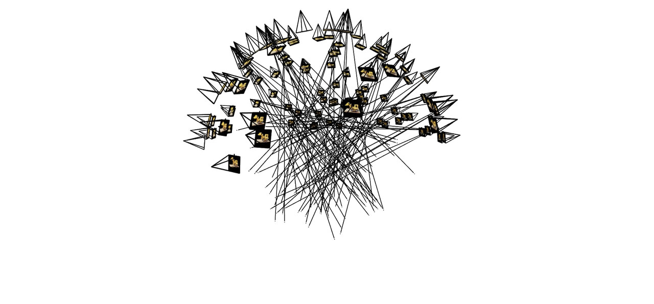
We use all the functions we made in the previous 2 parts to implement a custom dataset that takes in a set of images, corresponding c2w matrices, an intrinsic matrix K, a parameter M for how many images to sample in sample_rays, and a flag perturb to indicate wheter perturbation should be added. The dataset returns a tensor of shape (10000, 64, 3) for each iteration, i.e. 10,000 rays and 64 sample points along each ray as well as a rays direction tensor R~d~ and a pixels tensor, both of shape (10000,3) for feeding through the model. A visualization of how this sampling looks like for the set of multi-view lego truck images is shown below.

NeRF Architecture

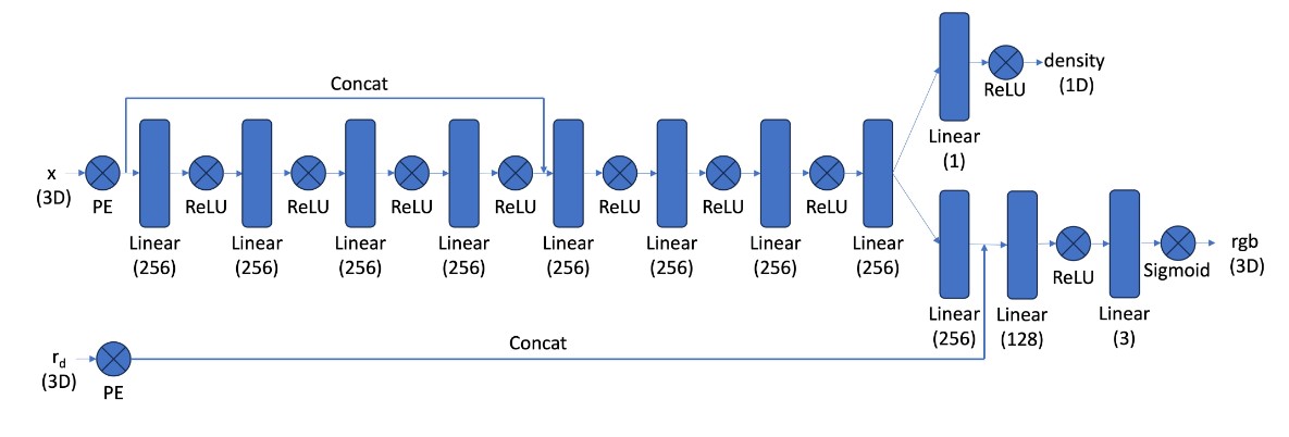
Now that all the preprocessing steps have been implemented, we create a neural network architecture that learns a mapping from 3D world coordinates and viewing direction to RGB values and density. We use the architecture shown below, which takes in two tensors, one containing world coordinates and the other ray directions (or viewing directions). These inputs are fed through many MLP layers to get a tensors of densities and RBG values [both of shape (batch_size,64,3)] at the end. Since we are representing a 3D space, which is much more complex than a 2D space, we need a deeper network to learn the function. Moreover, the skip connections serve to alleviate the vanishing gradient problem so the network doesn’t “forget” about the earlier layers and inputs. For positional encoding, we used L=10 for the x tensor of world coordinates and L=4 for the r~d~ tensor of ray directions.

Volume Rendering

After getting the output tensors from the model, we need to translate the density and RGB information for each sample to a single RGB value for each ray. We do this via the volume rendering equation shown below, which sums up the RGB values for each sample along the ray according to their corresponding density to get a single RBG value for the ray at the end. We vectorize this equation using torch.cumsum and other torch operatations and make it a part of the NeRF model. So our model actually returns a tensor of shape (batch_size,3) containing the predicted RGB values for each ray

Results

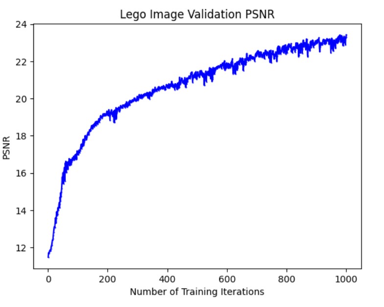
The PSNR curve on the validation set for the first 1000 training iterations and the predicted images for the first validation image on the iterations 1,50,100,200,500,1000 are shown below

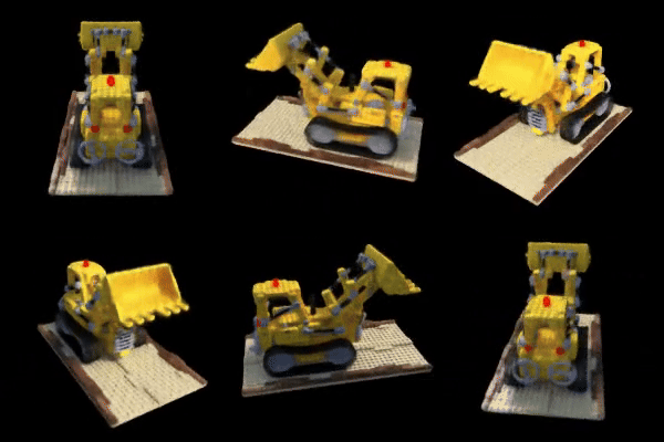
Running our trained model on the c2ws_test extrinsics provided allows us to produce 60 frames of the lego truck image rotating counterclockwise. We merge these frames to render a video

Bells & Whistles

Depth-Rendered Video

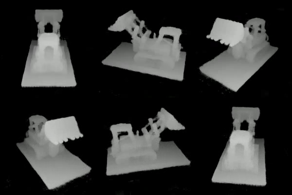
We also rendered a depths-map video by replacing the per-point color vector in the volume rendering equation with a scalar representing the depth of the point along the ray. Namely, the depths along the ray are represented by linspace(1,0,64), 64 evenly spaced depths from 0 to 1, one for each point. This gives the depth-map video below:

Color-Rendered Video

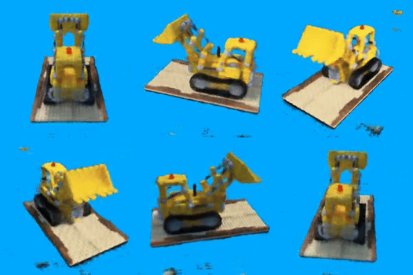
Finally, we rendered a video of the lego truck with a different background color by calculating 1 - sum(T~i~*(1-exp(σ~i~δ~i~)))*color for each ray, where color is a tensor of shape [3] containing the RGB value for the background color. We then add this to the tensor of colors that were rendered normally to get an image with the background color changed. Conceptually, this works because it is tantamount to adding the expected value that the ray is a background ray with color color, which is just the probability that the ray doesn’t terminate at any of the points multiplied by color. After making this change to the volume rendering equation, we can change the background color of the lego image as shown below:

Conclusion

Neural Radiance Fields are an incredible approach to represent 3D spaces and render multi-view images using neural networks. Though the model is computationally expensive and requires a large amount of data, its ability to generalize to unseen perspectives makes it a great approach for computer vision tasks.

References

1. Mildenhall, B., et al. (2020). NeRF: Representing Scenes as Neural Radiance Fields for View Synthesis. In Proceedings of the European Conference on Computer Vision (ECCV). 2020.
2. Tancik, M., et al. (2020). Fourier Features Let Networks Learn High Frequency Functions in Low Dimensional Domains. Advances in Neural Information Processing Systems (NeurIPS).