Background

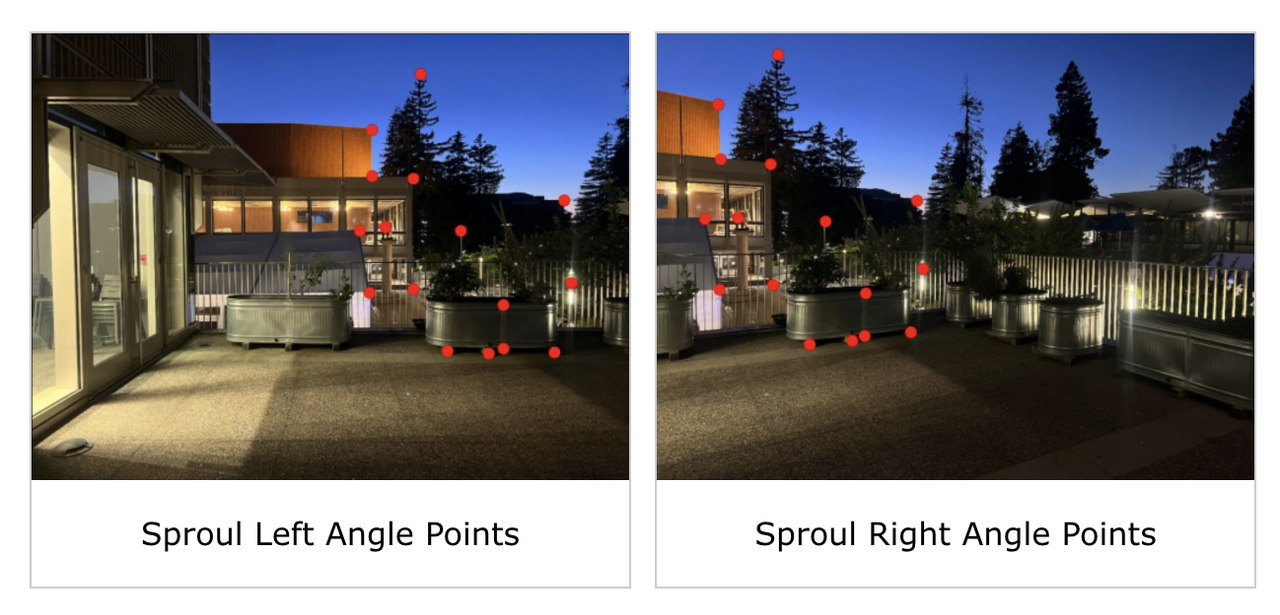
In this part of the project, I explore some interesting applications of image homography like rectification and mosaicing. I derived a least squares solution to the homography matrix and shot pictures of various objects and environments at my house and on the UC Berkeley Campus which I compute the homographies on.

Shooting the Pictures

I shot the pictures in this project using my iPhone Camera (iPhone 13 Pro Max) which gave me an initial size and resolution of 4032x3024. However, this size was too large so I later downsampled it to a size of 1200x900 to make computations faster. Furthermore, I used focus and exposure locking (AE/AF) to ensure the settings don’t change across perspectives

Recovering Homographies

We want to recover a 3x3 homography matrix, H, from one set of points to another. Because we have 8 unknowns in H, only 4 pairs of correspondence points are needed to recover it. However, using 4 points makes H unstable and prone to noise so it’s better to have more points and find the best solution using least squares. We can write out an overdetermined system of equations between the correspondence points and find a least squares setup to recover H.

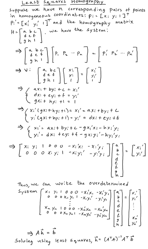
Image Rectification

Having found a way to recover the homography matrix, we can “rectify” images, i.e. warp them so the plane is frontal-parallel. Because we have only one image, we find an object in that image we know is rectangular and define two sets of points: one being the corners of the rectangular object in the image and the other a manually defined forward-facing rectangle in the image plane. Then, we compute the homography between these set of points and warp the image via this homography to make it frontal-parallel. This has the effect of changing our perspective angle on the image

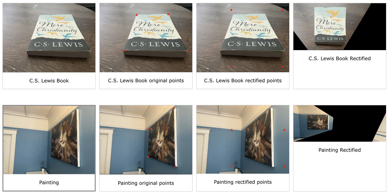
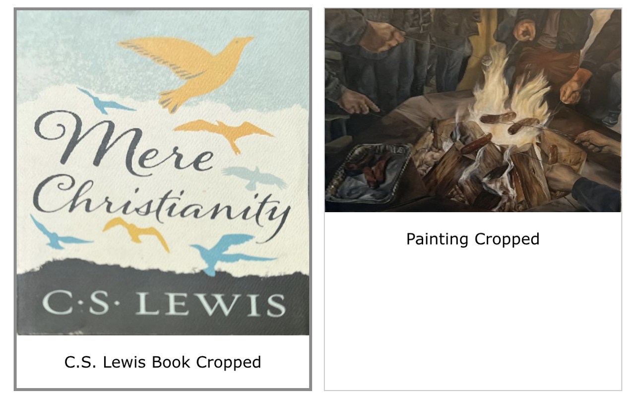
It’s pretty cool that even though the pictures are taken at an angle, we can recover a full-frontal view of the image. Below are the cropped versions of the rectified book and painting images. Notice that we have a much clearer front-facing view of the book and painting than in the original images

Blending Images into a Mosaic

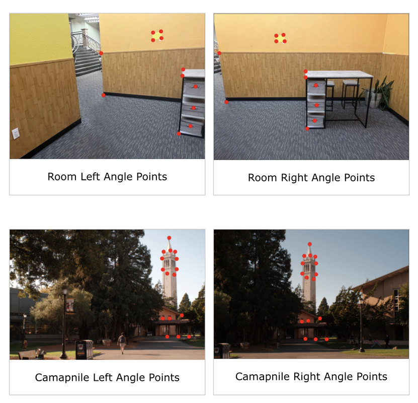
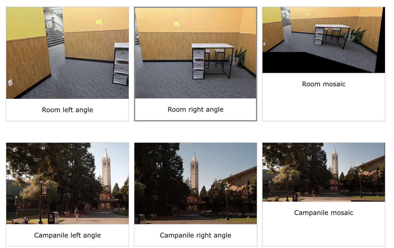
Using homography, we can also blend multiple images into a mosaic that covers a wider field of perception. Given a set of images and correspondence points from left to right, my procedure for creating a mosaic was first warping each image except the leftmost one into the leftmost one via a homography. Then, we have a set of warped images of the same size (with the actual image in different locations on the plane) that need to be stitched together. I tried many different blending techniques like laplacian pyramids and gaussian alpha channels but the technique that seemed to work best was using a linear gradient mask in the overlapping region. To stitch two images together, this involved first calculating the overlapping region then creating a linear gradient mask that goes from 1 to 0 in this region column-wise. Then I create a left mask and a right mask, where the left mask contains the area of the left image but replaced with the linear gradient mask in the overlapping region and the right mask contains the area of the right image but replaced with the inverse of the linear gradient mask (goes from 0 to 1 instead) in the overlapping region. Then, I calculated the stitched image as left_maskleft_image + right_maskright_image. This has the effect of keeping the left and right images in regions where they are exclusive but creaing a smooth transition from the left to the right in the region they overlap. I found that this technique also elimiates edge artifacts which were common in the other techniques I explored.

Project 4 Part B: Feature Matching for Autostitching

Background

In part B of this project, I create a system for automatically stitching images into mosaics, without requiring human input for point correspondences. We largely follow the algorithm outlined in this paper Multi-Image Matching using Multi-Scale Oriented Patches by Brown et al. which involves detecting the harris corners, using adaptive non-maximal suppression to restrict and ensure the points are spatially well-distributed, extracting and matching feature descriptors for each point, and finally using RANSAC to compute a robust homography estimate between the images. At the end, I show some examples of images that were automatically stitched using this method

Detecting Harris Corners

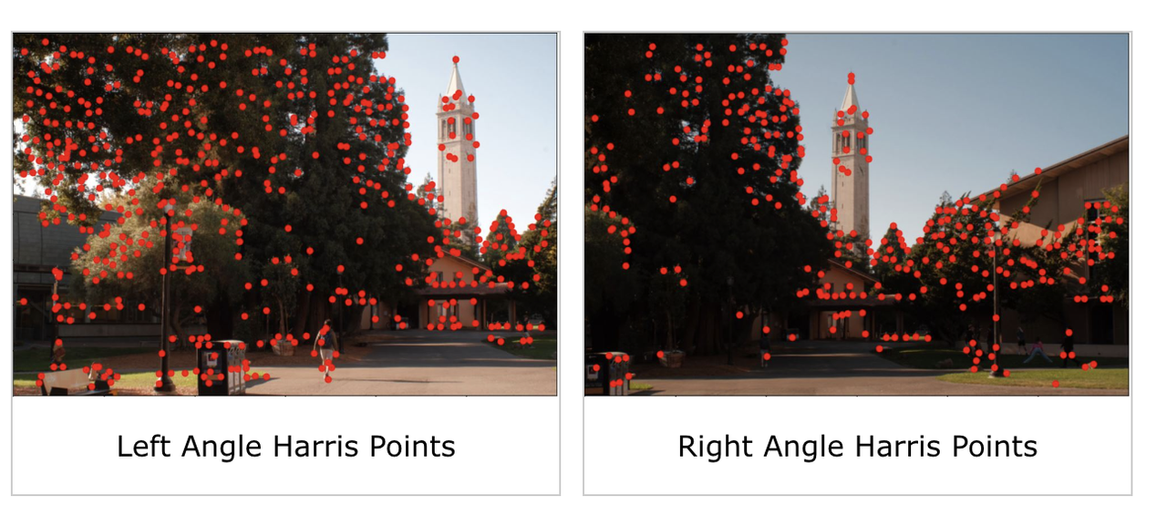
First, we need to find salient features in each image so we have something good to match. We use the Harris detector to find corners in each image. The detector identifies corners by testing the change in intensity across the different directions from a point. If the point is a corner, it changes significantly in intensity across multiple directions. If it changes significantly in only one direction, the point is on an edge.

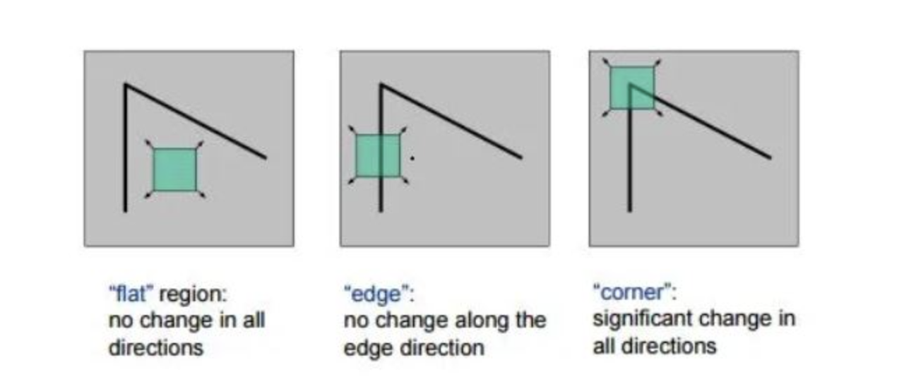
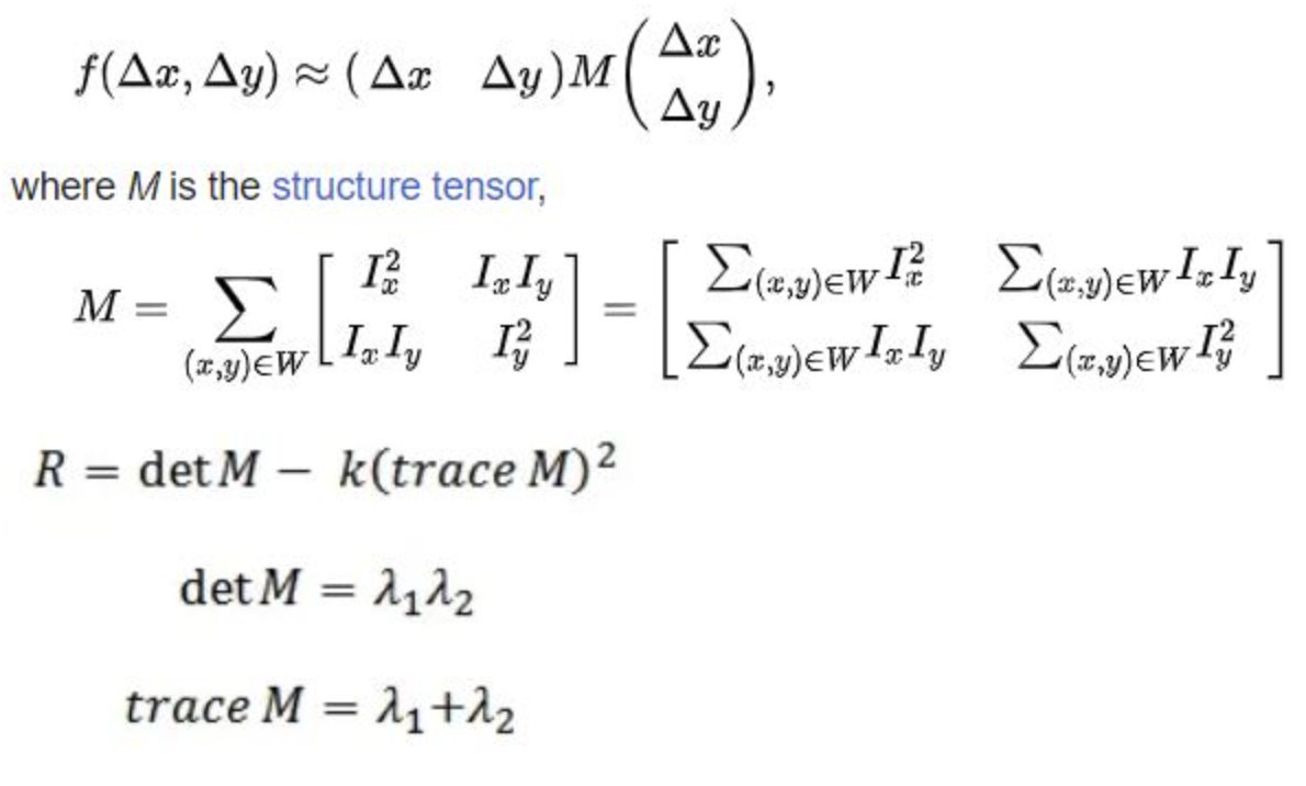
Mathematically, we find the SSD between an image patch around the original point and a patch around the shifted point. We can approximate this SSD using matrix Taylor expansion to get the equation below. Finally, to calculate the response for a point, we use the response equation below. When R is large and postive, both eigenvalues are large, meaning the SSD has large shifts in all directions and the point is a corner. We implement Harris Corner Detection using the provided harris.py code.

Adaptive Non-Maximal Suppression

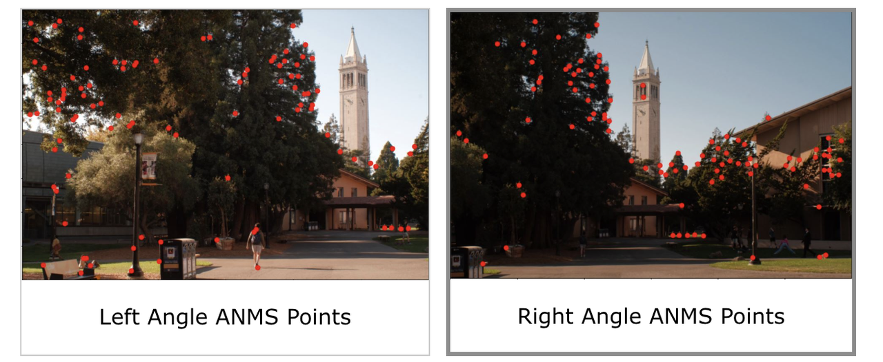
Because the computational cost of matching is high, it is beneficial to restrict the number of interest points used. However, we also want to ensure that the points are spatially well-distributed since the area of overlap between two images may be small. Therefore, we use the adaptive non-maximal suppression algorithm outlined in the paper to select a smaller number of interest points for the image. The algorithm works by calculating a radius, r_i for each interest point by finding the distance to the closest point in a 3x3 window whose harris response is sufficiently higher than the interest point’s response. Then, we take the n interest points with the highest radii. This ensures we only reject points with small radii, which are already “covered” by other interest points. For this project, I used n = 100 points

Extracting Feature Descriptors

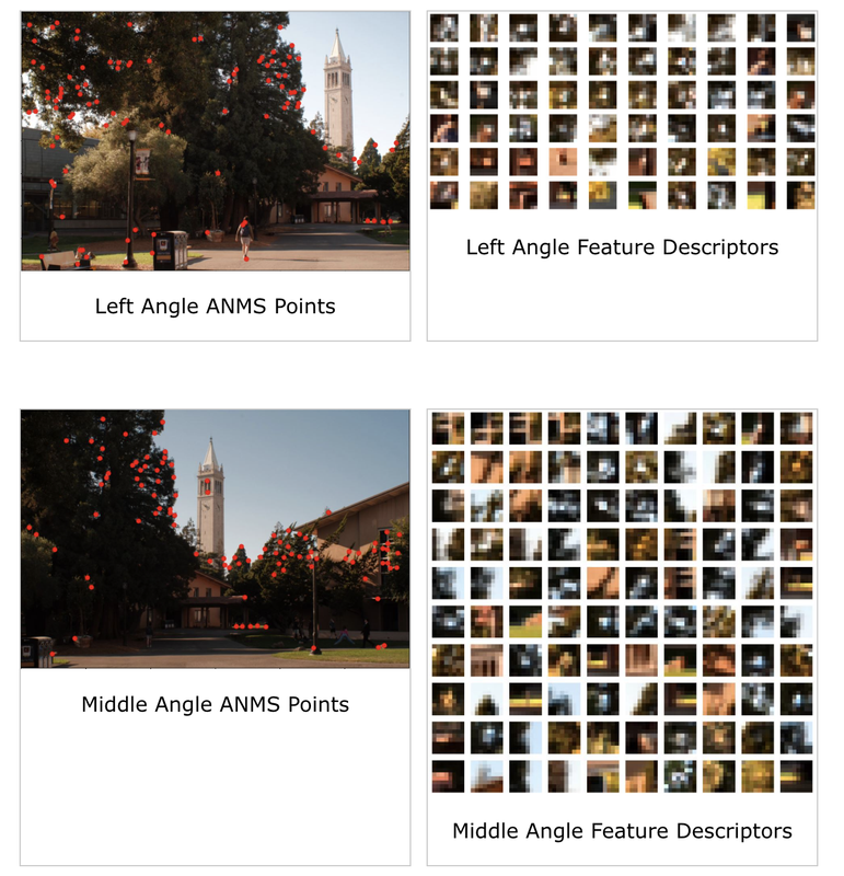
Now that we have interest points for each image, we can compute feature descriptors for each point to be used in matching later. Again following the paper, we compute a feature descriptor for an interest point by taking a 40x40 image patch around the point and rescaling it to a size of 8x8. We then normalize the entire patch so it has a mean of 0 and standard deviation of 1. This makes the descriptors have consistent computations when we later match them. In the feature descriptor images below, each feature descriptor was re-normalied to be between 0 and 1 for viewing purposes

Matching Feature Descriptors and Outlier Rejection

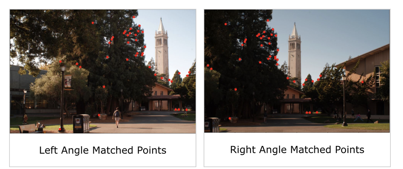
Next, we match the feature descriptors across two images to come up with a robust selection of point pairs. For matching, we use the nearest neighbors method (NN) with Lowe thresholding. For each point p in the first image with feature descriptor f~p~, we calculate the SSD with every feature descriptor in the other image, recording the smallest (p_1_nn) and second-smallest (p_2_nn) matches. Then, we reject p if p_1_nn/p_2_nn > ε for some threshold ε because this would mean p does not have many strong matches in the other image so it probably doesn’t lie in the overlapping area. If p is not rejected, we match it with its nearest neighbor in the other image and remove that neighbor from the other image’s set of interest points so that we do not have a double match to the same point. We perform this process for every interest point in the first image. At the end, we are left with a set of point correspondences between the two images

Homography via RANSAC

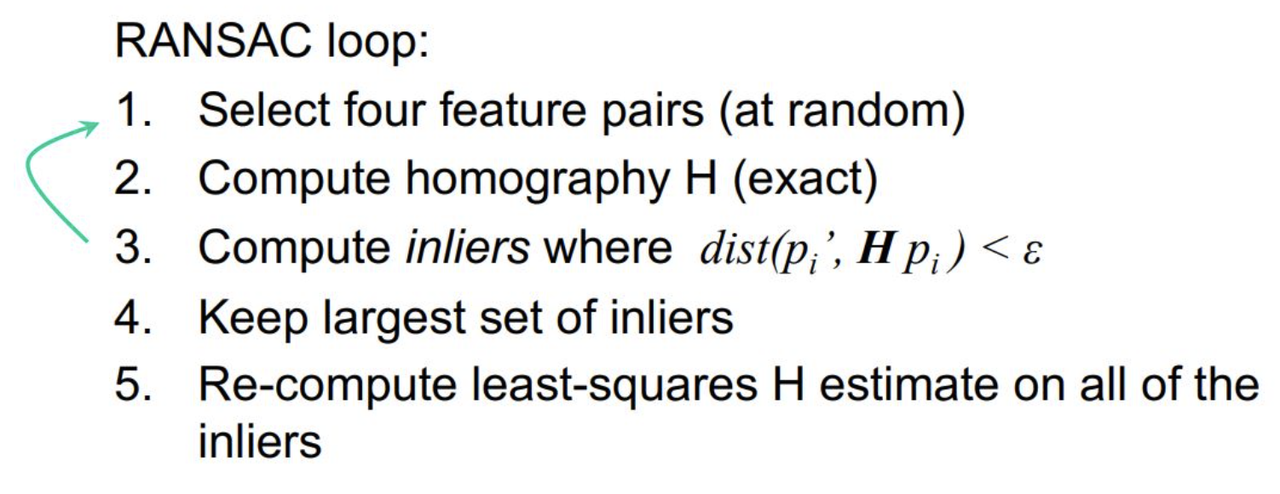
The last part of the process is to compute a robust homography estimate between the two images using the point correspondences we derived. To do this, we use the RANSAC algorithm. We randomly select 4 point pairs between the images and compute an exact homography estimate on these pairs (since the homography matrix has exactly 8 unknowns). Then we count the number of inliers, i.e. the number of point pairs that are described well by this homography matrix. We loop through these steps for some number of iterations (I used 1000 iterations), recording the largest set of inlier pairs found over all iterations. Finally, we compute a final homography estimate via least squares on this largest inliers set. RANSAC works because with enough iterations, there is a good chance that a well-defining set of 4 pairs is chosen at some point in the loop, especially with a lot of correspondences in the overlapping region. These 4 pairs would define a good homography estimate which is later refined by least squares.

Autostitching Mosaics

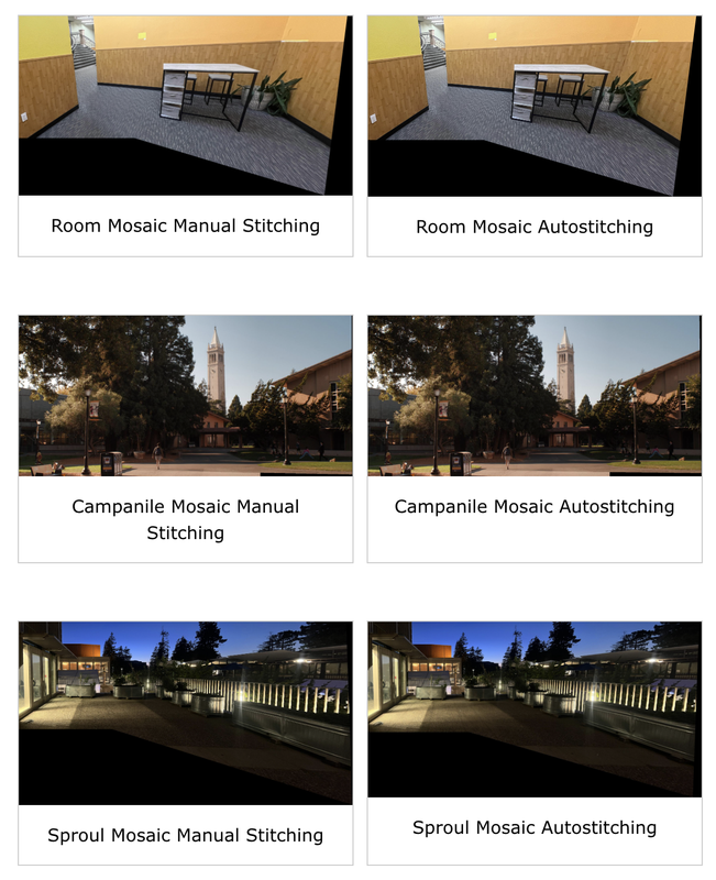
After automatically computing a homography between two images, we can warp them and stitch them together to form a mosaic. We perform this autostitching on the 3 sets of images we used for mosaics in the previous part. We also apply the same gaussian mask blending we used in the previous part to ensure a smooth transition between images and no edge artifacts

Conclusion

Overall, this was an interesting project and I enjoyed working through it, though the image stitching portion of image mosaicing was quite cumbersome :(. A cool thing I learned is that homographies cannot “create” information. A lot of times, I expected the homography to make it look like I actually changed perspective but this would require additional information that isn’t in the image. The homography simply lets us warp the image to make it look as close to shifting perspective as possible without adding information.